[超譯]ThinkDSP 第二章

第二章 諧波 | Harmonics

在這章，我會介紹幾個新的波形，我們會看到他們的頻譜以瞭解他們的諧波結構，那是由一組正弦曲線組合而成。
我也會介紹在數位訊號處理中最重要的現象之一：aliasing。我也會較仔細解釋 Spectrum 類別是怎麼運作的。
這章的程式碼在 chap02.ipynb，它的位置請看0.2節。也可以在這裡找到 http://tinyurl.com/thinkdsp02

2.1 三角波 | Triangle waves

一個正弦曲線只有一個頻率組成，所以它的頻譜只有一個尖峰。較複雜的波形，像是小提琴錄下來的，經由 DFT 之後，會得到多個尖峰。在這節，我們會探討波形與頻譜之間的關係。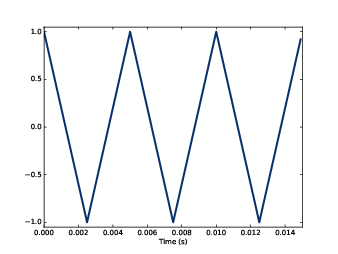

---

圖2.1：200 Hz 的三角波的片段

---

我會從一個三角波開始，它就像是正弦波的直線版。圖2.1 就是一個三角波，它的頻率是 200 Hz。
要產生一個三角波，可以使用 thinkdsp.TriangleSignal：

class TriangleSignal(Sinusoid):

    def evaluate(self, ts):
        cycles = self.freq * ts + self.offset / PI2
        frac, _ = np.modf(cycles)
        ys = np.abs(frac - 0.5)
        ys = normalize(unbias(ys), self.amp)
        return ys

TriangleSignal 從 Sinusoid 繼承了 __init__ 所以它也有同樣的參數 freq、amp 及 offset。
唯一的差別是 evaluate。就如我們之前看到的，ts 是取樣時間的序列，那些時間是我們要評估訊號的。
有許多方法可以產生三角波，細節不是非常重要，但以下是 evaluate 的運作：

1. cycle 是從開始時間到現在有幾個循環(cycle)。np.modf 會把 cycle 的小數部份放在 frac，整數部份則會忽略。[譯註：在解釋 evaluate 的第二行]
2. frac 是一個序列，裡面的每個值都是給定的頻率的斜率，值在 0 到 1 之間。減去 0.5 之後，範圍變成 -0.5 到 0.5。取絕對值得到一個波形是在 0.5 與 0 之間的之字型移動。
3. unbias 移動波形往下，所以讓它的中心在 0。接下來則是正規化，讓它可以符合給定的振幅 amp。

以下是產生圖2.1 的程式：

signal = thinkdsp.TriangleSignal(200)
signal.plot()

---

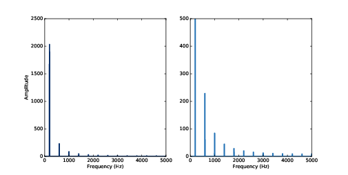
圖2.2：200 Hz 三角波的頻譜，兩邊的垂直軸是不同範圍。右方的圖讓基頻振幅被圖切掉，是為了讓諧波更為清楚。

---

接下來我們使用 Signal 產生 Wave，然後用 Wave 產生 Spectrum：

wave = signal.make_wave(duration=0.5, framerate=10000)
spectrum = wave.make_spectrum()
spectrum.plot()

圖2.2 顯示了兩個不同尺度的結果。右方的圖是為了讓諧波比較清楚而做了尺度上的調整。如預期，最高的尖峰是基頻 200 Hz。而且還有其他的尖峰在諧波頻率，它是 200 的整數倍。
但是有一個驚寄的地方是，偶數倍的 400、800 等等卻沒有尖峰。三角波的諧波都是在基頻的奇數倍，以本例來說，在 600、1000、1400 等等。
這個頻譜還有另一個特色是振幅與諧波頻率之間的關係。它們的振幅下降正比於隨頻率平方。比如說，前兩個諧波(200 與 600 Hz)頻率比是 3，振幅比則接近 9。接下來兩個諧波(600 與 1000 Hz)的頻率比則是 1.7，振幅比接近 1.7 的平方 2.9。這樣的關係叫諧波結構。

2.2 方波 | Square waves

---

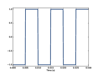
圖2.3：100 Hz 方波的片段

---

thinkdsp 也提供 SquareSignal 這代表一個方波，接下來是此類別的定義：

class SquareSignal(Sinusoid):

    def evaluate(self, ts):
        cycles = self.freq * ts + self.offset / PI2
        frac, _ = np.modf(cycles)
        ys = self.amp * np.sign(unbias(frac))
        return ys

SquareSignal 也從 Sinusoid 繼承了 __init__，所以參數也一樣。
evaluate 方法的內容也相似，cycle 仍是從時間開始算有幾個循環，frac 是小數部份，它是每個週期的斜率從 0 到 1。
unbias 移動 frac 讓斜率從 -0.5 到 0.5，然後 np.sign 讓負值全變成 -1，正值全變成 1。最後乘上 amp 得到方波的振幅在 -amp 到 +amp 之間。

---

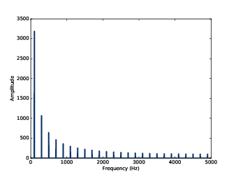
圖2.4：100 Hz 方波的頻譜

---

圖2.3 顯示方波的三個週期，圖2.4顯示它的頻譜。
跟三角波一樣，方波也只包含奇數諧波，所以尖峰在 300、500、700 Hz 等等。但諧波的振幅下降比較緩慢，嚴格來說，振幅下降正比於頻率(不是頻率平方)。
最後這章的練習給你個機會探索其他的波形與諧波結構。

2.3 混疊 | Aliasing

---

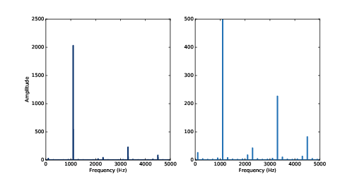
圖2.5：1100 Hz 三角波的頻譜，framerate 是 10000。右方的圖經過尺度調整以顯示諧波

---

其實我藏了一手，我在前面章節的範例是精心挑選的，以避免讓你混亂。但現在是時候該讓你混亂一陣子。
圖2.5 顯示 1100 Hz 三角波的頻譜，每秒取樣 10000 次。右方的圖經過尺度調整以顯示諧波。
它的諧波應該在 3300、5500、7700、9900。在這圖裡，如預期在 1100、3300 Hz 有尖峰。但第三個尖峰在 4500，而不是 5500 Hz。第四個尖峰在 2300 而不是 7700 Hz。如果你仔細看，應該在 9900 的尖峰出現在 100 Hz。這是怎麼回事？
這問題是，當我們 evaluate 訊號的時候，是時間上的離散的點，其實在點與點之間的訊息是不知道的，對於低頻成份，還不是個問題，因為在每個週期之間有很多取樣點。
但是，如果你在 5000 Hz 的訊號，取樣只有每秒 10000，那麼每週期只有兩個取樣點。很勉強的說是足夠。但如果頻率再高一點，就不行了。
來看為什麼。我們來產生 cosine 訊號，頻率為 4500 與 5500 Hz。然後取樣率為每秒 10000 次：

framerate = 10000

signal = thinkdsp.CosSignal(4500)
duration = signal.period*5
segment = signal.make_wave(duration, framerate=framerate)
segment.plot()

signal = thinkdsp.CosSignal(5500)
segment = signal.make_wave(duration, framerate=framerate)
segment.plot()

---

圖2.6：4500 Hz 與 5500 Hz 的 cosine 訊號，在取樣率 10000。訊號是不同的，但取樣之後卻長得一樣。

---

圖2.6 顯示了結果，我把訊號用淡灰色線畫出來，把取樣值用垂直線畫，是為了要讓兩個波形容易比較。這問題很明顯，就算訊號不同，但取樣之後兩個波形畫出來一樣。
我們對 5500 Hz 訊號用 10000 的取樣率得到的結果跟 4500 Hz 的結果是分不出來的。同樣 7700 Hz 與 2300 Hz 的結果也是分不出來，9900 Hz 與 100 Hz 也是。
這個效應叫做 aliasing，因為高頻訊號被取樣時，他變得跟低頻的一樣。
在這個例子，10000 取樣率的一半是 5000，就是我們可取率的最高頻率。超過 5000 的頻率，就會被折掉 5000 Hz。這個取樣率的上限就因此叫做折疊頻率。它有時也被叫做 奈奎斯特頻率。請參閱 http://en.wikipedia.org/wiki/Nyquist_frequency
如果 aliasing 頻率被折到低於 0，這折疊頻率要再繼續折。例如，1100 Hz 的三角波的第 5 個諧波是在 12100 Hz，折疊頻率是 5000 Hz，那它應該出現在 -2100 Hz，但它應該對 0 Hz 折一次，就變成出現在 2100 Hz。事實上，在圖2.4 裡你可以看到有個小尖峰在 2100 Hz，再下一個是在 4300 Hz。

2.4 計算頻譜 | Computing the spectrum

我們已看過 Wave 的 make_spectrum 方法好幾次，現在來看它的實作(有些細節後面會再說明)：
from np.fft import rfft, rfftfreq

 class Wave:
    def make_spectrum(self):
        n = len(self.ys)
        d = 1 / self.framerate

        hs = rfft(self.ys)
        fs = rfftfreq(n, d)

        return Spectrum(hs, fs, self.framerate)

這參數 self 是 Wave 物件自己。n 是 wave 物件裡，取樣點的數量。d 是取樣率的倒數，就是每個取樣點的時間間隔。
np.fft 是 numpy 模組裡的 Fast Fourier Transform (FFT 快速傅立葉轉換)，它是一個計算 Discrete Fourier Transform (DFT 離散傅立葉轉換) 的有效率的演算法。
make_spectrum 使用 rfft，它代表著 real FFT，因為 Wave 包含了實數，而不是複數。稍後我們會用 full FFT，這就可以處理複數訊號(參見 7.9節)。rfft 的結果我叫它為 hs，它是一個numpy 提供的複數的 array，它可用複數形式來表示波裡面每個頻率成份的振幅與相位移。
rfftfreq 的結果，我叫它為 fs，它是一個 array，裡面的值就是對應於 hs 所應該有的頻率。
要瞭解 hs 裡面的值，可以用兩個方法來思考複數：

• 複數是實部與虛部的和，通常寫在 $x + iy$。$i$ 是單位虛數 $\sqrt{-1}$，你可以把 $x$ 與 $y$ 想成卡式座標。
• 複數也可以看成 $A e^{i \phi}$ 這種形式，一個純數大小與複指數的相乘。A 是 magnitude，φ 是角度，單位是弧度，也叫做 argument。你可以把 $A$ 與 $\phi$ 想成極座標。

每個在 hs 的值，都對應到一個頻率成份，它的 magnitude 正比於對應的成份的振幅，它的角度是相位移。
Spectrum 類別提供兩個唯讀性質，amps 與 angles，它回傳 numpy array，代表 hs 的 magnitude 與 angle。當我們把 spectrum 物件畫圖時，我們通常畫的是 amps vs fs。有時畫出 angles vs fs 也有用。
雖然，有時會想看 hs 的實部與虛部，但你幾乎不需要這樣做。我鼓勵你用振幅與相位移的組合來想像 DFT 裡面的每個複數。
想要修改頻譜，你可以直接對 hs 處理，例如：

spectrum.hs *= 2
spectrum.hs[spectrum.fs > cutoff] = 0

第一行是把 hs 裡每個元素都乘 2，所有的成份的振幅都變成兩倍。第二行是把 hs 裡頻率超過 cutoff 的元素的值都設為 0。
但是 Spectrum 也有提供方法可做這些操作

spectrum.scale(2)
spectrum.low_pass(cutoff)

你可以到後面的網址看這些方法的文件：http://greenteapress.com/thinkdsp.html
到了這裡，應該你更了解 Signal、Wave、Spectrum 類別如何運作。現在還沒有解釋到 Fast Fourier Transform 是如何運作的，這還需要幾章的知識。

2.5 練習

這些習題的解答在 chap02soln.ipyb。
Exercise 1 If you use Jupyter, load chap02.ipynb and try out the examples. You can also view the notebook at http://tinyurl.com/thinkdsp02.
Exercise 2 A sawtooth signal has a waveform that ramps up linearly from -1 to 1, then drops to -1 and repeats. See http://en.wikipedia.org/wiki/Sawtooth_wave
Write a class called SawtoothSignal that extends Signal and provides evaluate to evaluate a sawtooth signal.
Compute the spectrum of a sawtooth wave. How does the harmonic structure compare to triangle and square waves?
Exercise 3 Make a square signal at 1100 Hz and make a wave that samples it at 10000 frames per second. If you plot the spectrum, you can see that most of the harmonics are aliased. When you listen to the wave, can you hear the aliased harmonics?
Exercise 4 If you have a spectrum object, spectrum, and print the first few values of spectrum.fs, you’ll see that they start at zero. So spectrum.hs[0] is the magnitude of the component with frequency 0. But what does that mean?
Try this experiment:

1. Make a triangle signal with frequency 440 and make a Wave with duration 0.01 seconds. Plot the waveform.
2. Make a Spectrum object and print spectrum.hs[0]. What is the amplitude and phase of this component?
3. Set spectrum.hs[0] = 100. What effect does this operation have on the waveform? Hint: Spectrum provides a method called make_wave that computes the Wave that corresponds to the Spectrum.

Exercise 5 Write a function that takes a Spectrum as a parameter and modifies it by dividing each element of hs by the corresponding frequency from fs. Hint: since division by zero is undefined, you might want to set spectrum.hs[0] = 0.
Test your function using a square, triangle, or sawtooth wave.

1. Compute the Spectrum and plot it.
2. Modify the Spectrum using your function and plot it again.
3. Use Spectrum.make_wave to make a Wave from the modified Spectrum, and listen to it. What effect does this operation have on the signal?

Exercise 6 Triangle and square waves have odd harmonics only; the sawtooth wave has both even and odd harmonics. The harmonics of the square and sawtooth waves drop off in proportion to 1/f; the harmonics of the triangle wave drop off like $1/f^2$. Can you find a waveform that has even and odd harmonics that drop off like $1/f^2$?
Hint: There are two ways you could approach this: you could construct the signal you want by adding up sinusoids, or you could start with a signal that is similar to what you want and modify it.
註1：python 裡，用 _ (底線) 當變數名稱是一個習慣用法，通常用在「我不想要用這個變數值」的情況。